The loss breakdown
Every component of the performance ratio — inverter, cables, soiling, temperature, mismatch, shading, availability, transformer and other — with defaults and ranges.
The performance ratio — PR — is the fraction of the energy a plant would
generate if every module always ran at its nameplate efficiency that it
actually delivers to the grid. It is dimensionless, always below 1, and it is
the single multiplier that turns annual in-plane irradiance into specific yield:
Specific yield = GTI × PR. See
How yield is calculated.
You never type a performance ratio. There is no PR field. The application builds it from the components below, which means a PR you report is always traceable to a component you set — and a PR someone challenges can be answered component by component instead of defended as a single number.
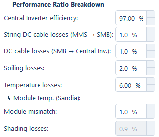
The full breakdown
Rows in the order they appear in the panel.
| Field | Default | Range | What it does |
|---|---|---|---|
| String Inverter efficiency | 97.0 % | 50–100 % | DC to AC conversion efficiency of the inverter. A factor, not a loss — a higher number is better. Reads Central Inverter efficiency in Central Inverter mode. |
| String DC cable losses | 1.0 % | 0–20 % | Resistive loss on the DC conductors between the module tables and the equipment that collects them. |
| AC cable losses (Str. Inv. → ICR) | 1.0 % | 0–20 % | Resistive loss on the run from the inverter to the inverter control room. Relabelled in Central Inverter mode — see below. |
| Soiling losses | 2.0 % | 0–20 % | Light blocked by dust, dirt and bird droppings on the glass. |
| Temperature losses | 6.0 % | 0–20 % | Power lost because modules run hotter than their rating condition. Computed, not assumed, once a module file is loaded. |
| Module mismatch | 1.0 % | 0–10 % | Loss from modules in one string not being electrically identical. |
| Shading losses | 1.0 % | 0–20 % | Row-to-row near-shading. Computed by default. Editable only when auto-compute is switched off. |
| Auto-compute (row-to-row from GCR) | on | — | When ticked, the shading figure is derived from your own row geometry rather than taken from the field above. |
| Module ground clearance | 0.5 m | 0.0–5.0 m | Height of the module's lower edge above ground. Drawing input for the shadow view only — it is not a loss and it does not change the computed shading figure. |
| Availability | 99.0 % | 50–100 % | Fraction of the year the plant is available to generate. A factor, like inverter efficiency. |
| Transformer losses | 1.0 % | 0–10 % | Copper and iron loss in the step-up transformer. |
| Other losses | 2.0 % | 0–10 % | Monitoring, auxiliary consumption and anything not covered above. |
Two rows are stated as efficiencies and eight as losses; the auto-compute option and the ground clearance are neither. Read the units before changing anything: entering 97 in a loss field and 3 in an efficiency field describe the same physical inverter, and getting them the wrong way round moves the yield by a factor you will not notice in the summary.
How the components combine
Multiplicatively. The performance ratio is the product of every factor and of one minus every loss — it is not one minus the sum of the losses:
PR = (inverter efficiency / 100)
   × (1 − DC cable loss)   × (1 − AC cable loss)
   × (1 − soiling)         × (1 − temperature)
   × (1 − mismatch)        × (1 − shading)
   × (availability / 100)
   × (1 − transformer)     × (1 − other)
State it this way when the figure is reviewed, because it is the first thing a lender's reviewer asks and the two methods do not give the same answer. A product is always slightly higher than one minus the sum, and the gap widens as the individual losses grow: each loss applies to what the losses before it left, not to the full nameplate figure.
The monthly performance ratio is built the same way, with one substitution — the annual temperature loss is left out and a month-specific temperature loss put in its place, which is why monthly PR moves through the year while the other nine components stay put.
What changes with the electrical mode
Two labels follow the choice you made at launch, because the equipment the cables run between is different:
| Row | String Inverter mode | Central Inverter mode |
|---|---|---|
| Inverter efficiency | String Inverter efficiency | Central Inverter efficiency |
| First cable row | String DC cable losses | Relabelled to read MMS → SMB |
| Second cable row | AC cable losses (Str. Inv. → ICR) | Relabelled to read SMB → Central Inv. |
Three abbreviations run through those labels. MMS is the module mounting structure — the table the modules are bolted to. SMB is the string monitoring box, which collects strings in Central Inverter mode. ICR is the inverter control room, the building the collected power is brought back to.
The defaults and ranges are identical either way. See Choosing a design mode for what else the choice changes.
Component by component
Inverter efficiency
The DC to AC conversion efficiency of the inverter, entered as a percentage kept, not a percentage lost. A single figure stands in for the whole efficiency curve, so pick a weighted efficiency representative of how the plant will actually operate rather than the peak value from the top of the datasheet — a plant spends most of its energy-weighted hours below the peak.
An inverter file's main job elsewhere in the application is setting plant AC capacity, but its own efficiency curve is visible in the inverter file viewer, which is the place to read a representative figure from. See Inverter settings.
Loading an inverter file does not fill this field. The file sets the nominal and maximum AC power, updates the status line and recomputes the DC/AC ratio — and leaves the efficiency at whatever is already entered, which on a fresh session is 97.0 %. Open the file viewer, read a representative efficiency off the curve, and type it in yourself.
The two cable losses
Both are resistive losses, and what each one covers depends on the electrical mode. The routing behind them, and the lengths reported in the summary, are on Cable routing.
String DC cable losses covers the DC run from each module table to the string inverter serving it. The circuit needs a positive and a negative conductor, which is why the summary counts the DC conductor length as twice the routed path.
AC cable losses (Str. Inv. → ICR) covers the three-phase AC run from each string inverter to the nearest inverter control room.
Soiling
Light blocked by whatever settles on the glass — dust, dirt, bird droppings. The default of 2.0 % is a moderate figure. It is one of the few rows where local knowledge beats any general figure: a site near unpaved roads, cement works, or in a region with a long dry season and a monsoon that ends it carries a soiling loss that no default can represent, and cleaning frequency changes the answer as much as the site does.
If the design includes robotic cleaning, this is the row that should reflect it — see Robotic module cleaning.
Temperature
The one row that is a calculation rather than an assumption, as soon as a module file is loaded. It needs the module's temperature coefficient of maximum power, which is read from the file and typed nowhere in the panel. The computed module operating temperature is displayed beside the row and the working is shown underneath the inputs.
Without a module file it stays at 6.0 % and is an assumption like any other. The model, the four mounting configurations and the inputs that drive it are on Temperature loss.
Module mismatch
Modules within a string are never electrically identical — manufacturing tolerance, differing degradation, and small differences in operating condition mean the string operates at the current its weakest module allows rather than the average of all of them. The default of 1.0 % suits modules sorted into tight power bins.
Shading
Row-to-row near-shading: the shadow the row in front casts onto the row behind when the sun is low. Auto-compute (row-to-row from GCR) ships on, so by default this figure is derived from your own geometry — the ground coverage ratio (GCR) and the tilt — rather than taken from the field. GCR is the collector area divided by the ground area it occupies: here, the table height divided by the row pitch.
Switch auto-compute off and the field becomes editable, which is what you want when you are entering a figure from a dedicated shading study instead. Note that the automatic figure covers row-to-row shading only; terrain and horizon shading are not modelled. The full model and the shadow view that visualises it are on Shading loss.
Availability
The fraction of the year the plant is available to generate, entered as a percentage kept. It absorbs planned maintenance, forced outages and grid curtailment. The default of 99.0 % allows only a few days of unavailability across the whole year. A site with a weak grid connection, or one subject to a curtailment regime, does not deserve that number.
Transformer
Loss in the step-up transformer between the plant's AC collection voltage and the medium-voltage export. It is one figure for the transformer as a whole, so if your own loss schedule itemises no-load and load losses separately, combine them into this row rather than carrying one of them somewhere else as well.
Other
The catch-all: monitoring equipment, auxiliary consumption such as control-room supply and cooling, and anything else drawing energy that the rows above do not cover. At 2.0 % it is as large as the soiling allowance, so it is worth deciding deliberately rather than leaving it. If your own loss schedule itemises auxiliaries, put the itemised total here and note what it contains.
Module ground clearance
Module ground clearance is the height of the module's lower edge above the ground — not the height of the torque tube, the top edge, or the pile reveal. It ships at 0.5 m and accepts 0.0–5.0 m.
It sits among the loss rows but it is not a loss. Nothing is subtracted for it, and it does not appear anywhere in the performance ratio as a percentage.
The clearance does not enter the computed shading loss at all. The near-shading calculation is given the latitude, the tilt, the ground coverage ratio, the surface orientation and whether the plant is a tracker — and no clearance. Its only consumer is the cross-section drawn in the 🌓 Shadow View (row spacing) window. Changing it redraws that picture and leaves the Shading losses figure exactly where it was.
So treat it as what it is: a drawing input that makes the cross-section match the structure you are actually buying. Set it to the real lower-edge height of your mounting structure, and take the shading percentage from the row geometry that does drive it — the ground coverage ratio and the tilt.
Two of these rows are not assumptions
Eight of the ten loss and factor rows are inputs you own. Two are outputs of your design:
| Row | Derived from |
|---|---|
| Temperature losses | The module's temperature coefficient, the site's ambient temperature and wind speed, the mounting type, and the operating irradiance |
| Shading losses | Your own row geometry — the ground coverage ratio and the tilt, which follow from the table dimensions and the row pitch |
The consequence is worth stating explicitly, because it catches people comparing runs. Change the design and these two move on their own. Widen the row pitch and the shading loss falls. Load a different module and the temperature loss changes with its coefficient. Change the table height and both move, because the ground coverage ratio moved.
So when you compare two runs of the same site, expect eight rows to match and two not to. If all ten match after a geometry change, the design has not been put through the chain that derives them: the shading figure is produced when you Generate Layout, so generate again first and then click Calculate Energy. And when you hand a loss schedule to a third party, mark those two rows as computed rather than assumed, because they will not reconcile against a generic loss table and they are not meant to.
Where the breakdown is reported
The components are not only an input screen. When an energy calculation has been run, the exported report carries an energy section whose first page holds the energy inputs and this performance-ratio breakdown, component by component, beside the yield figures they produced. That page is the one to attach to a loss schedule, because it fixes which assumptions produced which number for a specific run rather than leaving the two to be matched up later. See PDF report.
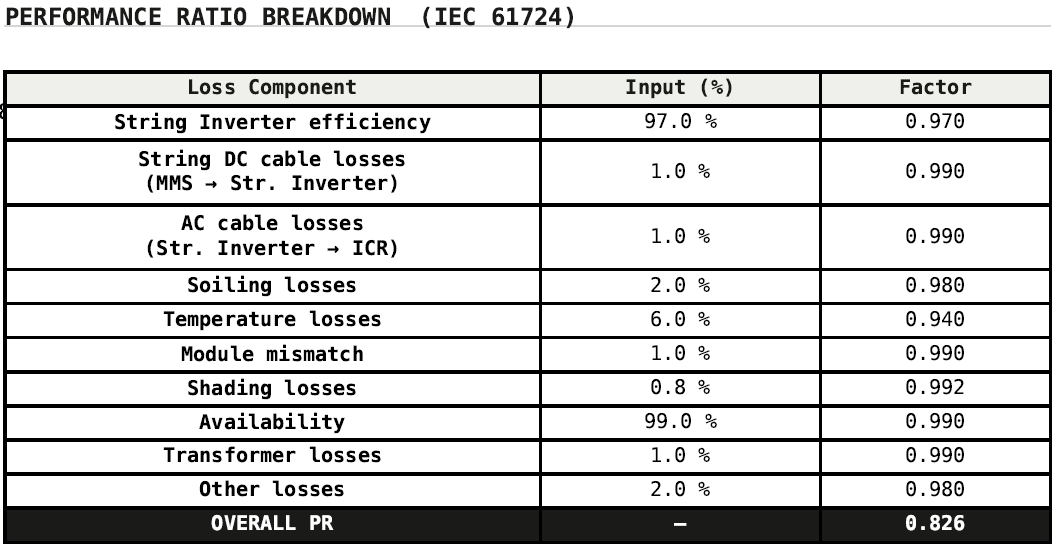
The performance ratio itself is not a summary-table column. What the summary carries is the result of applying it — the three probability columns, the capacity factor and the lifetime figure. See Summary columns.
Where to go next
Weather data
The automatic irradiance service and its fallback, your own hourly file and what it must contain, and how horizontal irradiance becomes in-plane.
Temperature loss
The thermal model behind the temperature row — module temperature from ambient, irradiance and wind, the four mounting types, and the loss it produces.