Your first layout
A complete first run — load a boundary, generate the layout, read the summary, calculate energy, and export the report.
This walkthrough takes one prepared boundary file and produces a placed plant, an energy estimate and a multi-page PDF report, changing almost nothing along the way. The point of a first run is to see what the defaults give you on your own site before you start fixing values.
It assumes Fixed Tilt with String Inverter, the combination most readers start from. Where a tracker plant or a central-inverter plant differs, the difference is noted — the full comparison is in Choosing a design mode.
Check what you need
Three things:
- The application, installed and open. The design-mode window appears first; pick Fixed Tilt with String Inverter.
- A valid licence for this machine. The application opens without one, and you can load a file and look at the inputs, but Generate Layout needs a valid, in-date licence. Glance at the access-status chip in the top toolbar first — it reads Active — until <date> when you're covered, or shows a Get Free Access / Contact Us button when you're not — or open Help ▸ License / Subscription… for the full detail before you start — see Activate your licence.
- One boundary file. A Google Earth file (
.kmzor.kml) with a closed boundary polygon is the easiest starting point. Water bodies, buildings and transmission lines drawn inside the boundary are read as exclusions.
If you are not sure your file is prepared correctly, read Preparing a Google Earth file first. A file whose boundary ring is not closed opens a Boundary Validation Issues window listing each problem boundary, with a checkbox to exclude it and carry on with the rest.
Load the boundary file
At the top of the input panel, the Input KMZ File row holds the path, a Browse… button, and an ⓘ button that opens the preparation guide.
Click Browse… and pick your file. The file window accepts
.kmz .kml .dxf .dwg .jpg .jpeg .png .gif .bmp .tif
.tiff.
What happens next depends on the kind of file:
| File | What you are asked |
|---|---|
.kmz or .kml | Nothing. The boundaries, obstacles and line features are read straight from the file, and the site's position comes with them. |
.dxf or .dwg | A DXF Site Coordinates window asks for the site latitude and longitude. They are optional — skip them and the layout is still generated, but energy calculation is unavailable. |
| An image | An Image Boundary — Scale & Coordinates window asks how a real site distance maps to a distance on the drawing, plus optional coordinates. The largest closed outline in the image becomes the boundary. |
Every feature in a Google Earth file must lie inside a boundary polygon.
Top-level polygons become plant boundaries; polygons fully inside one become
obstacles. Features are classified by name, case-insensitively — a polygon
named Pond or Reservoir is water, a line named 220kV or Powerline is a
transmission line and gets a corridor buffered either side of it, and a polygon
with no recognised keyword is a generic obstruction such as a building.
Look at the defaults that matter, and leave them alone
Every field below is already filled in. Read the values, confirm none of them is absurd for your site, and change nothing yet.
| Group | Field | Default |
|---|---|---|
| Module Specifications | Length (long side) | 2.38 m |
| Width (short side) | 1.13 m | |
| Wattage | 610 Wp | |
| Bifacial module | off | |
| MMS-Table Configuration | Orientation | Portrait |
| Modules per row | 28 | |
| Rows per MMS-Table | 2 | |
| Gap between modules E-W / N-S | 0.020 m each | |
| Gap between MMS-Tables | 1.0 m | |
| Maximize placement | off | |
| Add half tables in leftover space | off | |
| Spacing & Tilt | Override tilt angle | off — derived from latitude |
| Override row pitch | off — derived | |
| Site Parameters | Perimeter road width | 6.0 m |
| Place Lightning Arresters | off | |
| ICR Block | 18.0 MWp | |
| Transmission line corridor | 15.0 m per side | |
| String Inverter | Max strings per inverter | 20 |
| Calculate Cables for PV Power Plant | off |
Four of them decide the shape of the result:
Modules per row and rows per MMS-Table set the table itself. With portrait orientation, the module's short side runs east–west and its long side north–south, so the default table is 28 modules wide by 2 rows deep, with the gaps added between them. MMS is the module mounting structure — the rack the modules are bolted to. See Table configuration.
Perimeter road width decides how much ground you get. The plant boundary is shrunk inward by the perimeter road width to give the usable area; water bodies, obstructions, transmission corridors and any terrain exclusions are then subtracted from it. A table is placed only where it fits entirely inside what is left.
Tilt and row pitch are derived from the site latitude unless you tick the override boxes. The tilt follows a latitude rule of thumb; the row pitch is the spacing at which one row does not shade the row behind it at solar noon on the winter solstice. Neither is a value you have to supply for a first run, and seeing what the site's latitude implies is more useful than imposing a number. See Spacing and tilt.
ICR Block sets the capacity each inverter control room serves — an ICR is the inverter control room building. The number of control rooms is the plant capacity divided by this block size, rounded up.
Leave Calculate Cables for PV Power Plant unticked for a first run. Cable calculation is the slow step on a large or complex layout — tick the box and the application itself offers Enable Now and Not Now (Recommended). Inverter counts and capacities are computed either way; only the cable length columns stay blank. Generate first, review the layout, then enable it for the final run.
Click Generate Layout
The button sits below the input panel.
- What it shows
- The Generate Layout button with enough surrounding area to place it in the window.
- How to get there
- A boundary file loaded and a valid licence installed, so the button is enabled.
- Callouts to add
- Outline the button.
The application works through the site in a fixed order:
- The boundary file is read into boundaries, each carrying its own obstacles and line obstructions.
- Coordinates are projected into the site's local UTM zone, so all internal geometry is in metres.
- The boundary is shrunk inward by the perimeter road width.
- Polygon obstacles and the buffered transmission line and canal corridors are subtracted.
- Terrain exclusions are subtracted, when topography is enabled.
- The table grid is placed across what remains. Rows run east to west and panels face the equator — south in the northern hemisphere, north in the southern. A table is kept only where it fits entirely inside the usable area.
- Control rooms are placed. The tables are grouped spatially into blocks of roughly one capacity block each, and a control room sits at each group's centre, so every group of tables surrounds its own building. Tables overlapping a control room footprint are removed, and the control room count is then re-checked against the reduced capacity.
- String inverters are placed from clusters of tables, sited in the gap bands between rows, and cables are routed if you asked for them.
- Lightning arresters are placed, if you enabled them, and the capacity is recomputed.
A status line under the plot reports how many plants were laid out and the total area in acres. See How placement works for the detail.
Read the result
- What it shows
- The whole window after a successful fixed-tilt run on a single-plot site: the boundary, the placed tables, the control rooms, the legend, and the summary table filled in below the plot.
- How to get there
- Fixed Tilt + String Inverter, a single-boundary file of roughly 50 to 100 acres, defaults elsewhere. Maximise the window and press Home on the plot toolbar to fit the view.
- Callouts to add
- Number the boundary 1, a table 2, a control room 3, and the summary table 4.
On the plot: the plant boundary in gold, the module tables in blue, the control rooms in dark blue, the string inverters in green, water bodies in blue and other obstructions in red. The legend names them. Cables, terrain contours and arresters have their own switches and start off, so the first picture is the placement alone.
Under the plot, the Layout & Energy Summary carries one row per plant boundary and a TOTAL row across them. The columns you care about on a first run:
| Column | What it means |
|---|---|
Plant | The boundary's name, from the file |
Plant Area (Acres) | The plant area inside the boundary |
Plant Boundary (in meter) | The length of the plant boundary, in metres |
Full Tbl | Full MMS-tables placed |
Half Tbl | Half tables placed, if you enabled them — half the east–west width, carrying half the strings |
Modules | Total modules across the plant |
DC(MWp) | Installed DC capacity |
Tilt(°) | The tilt used. A trailing * means it was auto-calculated rather than entered |
Pitch(m) | The row pitch used, with the same * convention |
ICR | Inverter control rooms placed |
Str.Inv | String inverters placed |
Inv kWp | The capacity carried per string inverter |
A — in a column means the figure was not computed — the cable length columns
read that way until you turn cable calculation on. The ⛶ Maximize button on
the summary header opens the table in its own window, which is the only
comfortable way to read the full column set.
- What it shows
- The summary table after a multi-plot run with energy calculated, scrolled to show as many columns as possible, with the total row visible.
- How to get there
- Generate a multi-plot layout with cable calculation on, then calculate energy.
On a tracker plant, Full Tbl and Half Tbl read Full Trk and Half Trk,
and Tilt(°) becomes MaxAng(°). In central-inverter mode, Str.Inv and
Inv kWp are replaced by monitoring box and central inverter columns. The
complete list is in Summary columns.
Check the tilt and pitch the application derived
Scroll back to Spacing & Tilt. Both override boxes are still unticked, but the two labels beside them now report what the run actually used, and those values have been pre-filled into the greyed-out fields.
- What it shows
- The same group after Generate Layout has run — the two labels now report the derived values in green, and those values are pre-filled into the greyed-out fields.
- How to get there
- Generate a layout with both overrides left off, then look at the group again.
- Callouts to add
- Outline both green labels.
- The tilt comes from the site latitude, following the rule of thumb
tilt ≈ latitude × 0.76 + 3.1°. - The row pitch is the no-shading pitch at winter-solstice solar noon:
pitch = L·cos(tilt) + L·sin(tilt) / tan(solar elevation), whereLis the table's height in the tilt plane. - GCR — ground coverage ratio, the collector area as a fraction of the ground it occupies — is reported as the table height divided by the row pitch.
This is the moment to decide whether to take control. If your design fixes the tilt at a value the module supplier or the structure vendor has specified, tick Override tilt angle, type it, and generate again. The same applies to Override row pitch when the pitch is set by the tracker or table vendor, by a cleaning robot's reach, or by a land constraint. Tightening the pitch below the derived value raises the GCR and the capacity, and raises row-to-row shading with it.
Calculate energy
Energy is a separate step, and it needs the site's latitude and longitude — which a Google Earth file always carries, and a CAD drawing carries only if you supplied them.
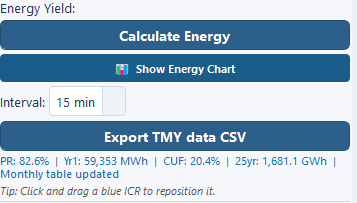
Click Calculate Energy. With the default weather source, PVGIS API (auto-fetch on Calculate), irradiance is fetched for the site from the EU Joint Research Centre service, with no key or account, falling back to NASA POWER when PVGIS has no data for the location. The GHI and in-plane GTI fields fill in with a label naming the source that was used. GHI is global horizontal irradiance; GTI is the irradiance in the plane of the modules.
Everything the estimate needs beyond irradiance is already set. The performance ratio — PR, the fraction of the theoretically available energy the plant actually delivers — is broken down loss by loss in the Energy Yield group, with the inverter at 97 %, soiling at 2 %, availability at 99 %, and row-to-row shading computed automatically from the GCR. Degradation ships at 1.0 % in the first year and 0.4 % a year after that, over a 30-year plant life. Change them when you have supplier figures; see Performance ratio and losses.
The results land at the right-hand end of the summary:
| Column | What it means |
|---|---|
P50Yr1(MWh) | Year-one generation at the first exceedance probability |
P75Yr1(MWh) | Year-one generation at the second |
P90Yr1(MWh) | Year-one generation at the third |
CUF(%) | Capacity utilisation factor — year-one energy against the plant running at full capacity all year |
25yrP50(MWh) | Cumulative generation over years 1 to Plant lifetime, at the first exceedance probability |
The three probability columns are named from the exceedance probabilities you set — 50 %, 75 % and 90 % by default — and the headers change with them. P90 is the figure a lender usually asks for: the annual energy the plant is 90 % likely to exceed.
The last column is the one to read carefully. Its header text is fixed, so it says
25yrP50(MWh) whatever you set, while the figure is the cumulative total over the
Plant lifetime — 30 years on the shipped default — at the first exceedance
probability. Quote it with the lifetime and the probability stated, not by its
header.
📊 Show Energy Chart draws the year as hourly bars for any day, or as twelve monthly bars with annual totals. Export TMY data CSV writes the full-year series at an interval you pick. Both are covered in Hourly and monthly output.
Export the PDF report
Click Export PDF (Layout + Summary). Every page is A3 landscape, in this order:
- Engineering drawing — the layout with a border, a north arrow, a title block, and a plant-details table with editable form fields.
- Summary — the layout summary, the design parameters, and the inverter and cable summary including the per-control-room cable breakdown.
- Single Line Diagram — your diagram, if you have built one.
- Bill of Material — paginated across as many pages as it needs.
- Energy — present only when an energy calculation has been run.
Export PDF (with Piles) produces the pile drawing instead, once you have defined a pile pattern under Edit-Pile ▸ Define Pile Layout….
Two other buttons carry the same layout elsewhere. Export KMZ writes the Google Earth file, with one folder per plant and a summary placemark. Export DXF writes the CAD drawing in UTM metres on named layers — boundaries, tables, control rooms, cables, trenches and annotations each on their own. See Exports.
Finally, save the session itself with File ▸ Save Project…. The project file holds the inputs, the layout, your hand edits, the diagram and the materials list, so you reopen exactly where you stopped. See Saving and reopening projects.
What to try next
Turn on cable routing
String, feeder and medium-voltage runs, with lengths and trench totals
Fit more into an awkward boundary
What Maximize placement and half tables buy, and what they cost
Edit the layout by hand
Move, copy and delete units, draw obstructions, annotate the drawing
Size the plant from an AC capacity
Work backwards from a target AC capacity and DC/AC ratio