Row-to-row shading
The computed row-to-row shading loss, the geometry behind it, the Shadow View cross-section, and what the model does not cover.
Row-to-row shading is the loss caused by each row of collectors casting a shadow onto the row behind it when the sun is low. It is the one loss in the performance ratio that is a direct consequence of your own layout decisions rather than of the site or the equipment: pitch, tilt and latitude fix it between them.
The application can either compute it from that geometry or take a percentage you enter. Computed is the default, and computed is what you should defend to a lender, because a fixed allowance carried over from another project has no relationship to the pitch you have actually drawn.
Two ways to set it
| Field | Default | Range | What it does |
|---|---|---|---|
| Shading losses | 1.0 % | 0–20 % | The annual shading loss applied to the performance ratio. Editable only when auto-compute is off |
| Auto-compute (row-to-row from GCR) | on | — | Computes the loss from the row geometry instead of taking the typed figure |
With auto-compute on, the Shading losses field is greyed out and the typed value is not what the calculation uses. Untick auto-compute and the field becomes editable, and the number you type is used exactly as entered.
Both fields sit in the performance ratio breakdown alongside the other loss components — see Loss breakdown.
The computed model
For parallel rows on flat ground, the shaded length s measured up the rear
collector is:
s/L = 1 − 1 / ( GCR · (cos β + sin β · cot ψ) )and the solar profile angle ψ in that expression is:
tan ψ = tan α / cos(γ_s − γ_c)Every term:
| Term | What it is |
|---|---|
s | The shaded length measured up the face of the collector behind, from its lower edge upward |
L | The collector slope length — the dimension of the collector measured up its tilted face, from lower edge to upper edge. Not the flat footprint the table occupies on the ground |
s/L | The shaded fraction of the rear collector: 0 is fully lit, 1 is fully shaded |
GCR | Ground coverage ratio — the collector width as a fraction of the row pitch. The application reports it as table height divided by row pitch, and it is the single number in which pitch enters this relation |
β | The collector tilt angle from horizontal — the tilt derived from latitude, or your override |
ψ | The solar profile angle — the apparent elevation of the sun as seen in the vertical plane perpendicular to the row axis. This, not the true solar elevation, is what decides how far a shadow reaches across the pitch |
α | The true solar elevation angle above the horizon |
γ_s | The solar azimuth — the compass direction of the sun |
γ_c | The collector azimuth — the direction the collector faces, which is the equator: south in the northern hemisphere, north in the southern |
γ_s − γ_c | How far the sun is round from straight in front of the array. At solar noon it is zero and the profile angle equals the solar elevation; morning and evening it grows, the profile angle collapses, and shadows run long |
Read the relation and the behaviour follows. The bracketed product
GCR · (cos β + sin β · cot ψ) has to exceed 1 before there is any shading at
all; below that the result is negative and the rear row is clear. As the sun
drops, cot ψ grows, the product grows past 1, and the shaded fraction climbs
from the lower edge of the rear collector upward.
Evaluated for every hour of a year
The relation above is an instantaneous geometric result for one sun position. It is not applied once at a design condition. Instead it is evaluated for every hour of a representative year, weighted by the in-plane beam irradiance at that hour, and returned as an annual beam near-shading loss in per cent.
Three things follow from that, and all three matter when the figure is challenged:
- The weighting is by beam, not by total irradiance. Beam irradiance is the direct component arriving straight from the sun's disc; diffuse is the rest, scattered by sky and cloud. Only the beam component casts the geometric shadow this model describes, so an hour with a high beam share counts for more than an overcast hour at the same sun position.
- Hours with no beam contribute nothing. A shadow geometrically present before dawn or under thick cloud carries no weight, which is why the annual figure is very much smaller than the worst-case instantaneous shaded fraction.
- The result is a single annual percentage, applied in the performance ratio like any other loss.
What the figure responds to
Because the loss is derived rather than assumed, it moves when the design moves:
| Change | Effect on the computed loss |
|---|---|
| Wider row pitch | GCR falls, the bracketed product falls, shading falls |
| Narrower row pitch | GCR rises, shading rises. This is the cost side of packing more capacity onto the site |
| Steeper tilt | Changes both cos β and sin β, and raises the collector, so the shadow reaches further at the same sun position |
| Higher latitude | The winter sun sits lower for more of the year, so the profile angle is smaller for more hours and the annual loss is larger for the same GCR |
| A different table geometry | Changes the collector slope length and therefore the GCR at a given pitch |
A fixed allowance cannot do any of this. Two plants at the same GCR but 20° of latitude apart do not have the same row-to-row shading loss, and the computed figure is the one that knows the difference.
Pitch is the lever with the most authority over this number, and it is set — automatically from latitude, or by your override — on Spacing and tilt.
When the figure is computed
The computed shading percentage is produced by Generate Layout, not by Calculate Energy. It is derived in the same pass that fills the derived tilt and the derived row pitch — which is the only pass that knows the geometry it needs.
Two consequences follow, and both catch people comparing runs:
- Calculate Energy consumes the figure; it does not produce it. By the time you calculate energy the shading loss is already fixed by the layout that was generated.
- Change the geometry and the figure is stale until you generate again. A new row pitch, a new tilt or a different table geometry moves the ground coverage ratio, and therefore the shading loss — but only once Generate Layout has run. Recalculating energy on its own leaves the old shading percentage in the performance ratio.
So the order is always the same: generate, then calculate energy. If you have changed anything about the rows, generate again first.
Overriding with your own figure
Untick Auto-compute (row-to-row from GCR) and the typed Shading losses value is used as entered. Legitimate reasons to do it:
- Your own detailed shading study, from a tool that models the horizon and the terrain, gives a figure you want carried through.
- A contractual or lender-mandated loss assumption has to be used for the case being reported.
- You are reproducing an earlier study built on a stated allowance.
An override does not change the Shadow View picture or the geometry — it only replaces the number entering the performance ratio. If your typed value and the computed value disagree substantially, one of them is describing a different plant. Find out which before reporting either.
The Shadow View window
🌓 Shadow View (row spacing) opens a two-dimensional cross-section of three adjacent rows, cut in the plane perpendicular to the row axis — the view you would get by standing at the end of a row and looking along it. Two sliders move the sun: one for the day of the year, one for the solar hour. The shaded part of each rear collector is highlighted live as you move them.
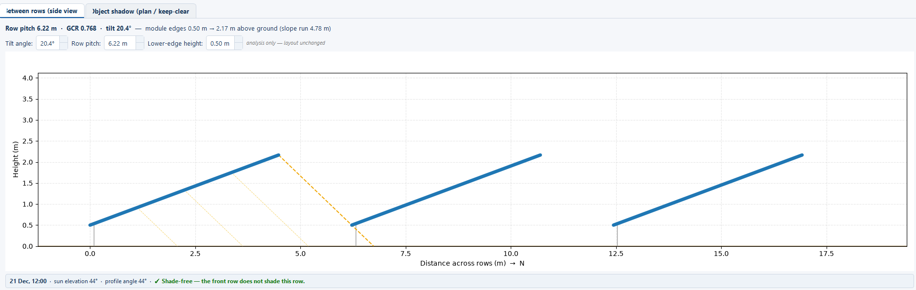
It is driven by the same model as the loss number, so the picture and the number always agree. The cross-section is not an illustration drawn to a different set of assumptions — it is the same geometry evaluated at the one sun position the sliders select, rather than summed over a year.
How to use it
Open it on a generated layout
The window needs the row geometry, so generate the layout first. The tilt and pitch it draws are the ones in force, whether derived or overridden.
Go to the worst case first
Drag the day slider to midwinter and the hour slider to early morning. That is when the sun is lowest and furthest round in azimuth, the profile angle is at its smallest, and the shadow reaches furthest across the pitch. If the rear collector is still substantially clear there, the design has real margin.
Sweep the day at a fixed hour, then the hour at a fixed day
Sweeping the day slider at a fixed early hour shows the seasonal swing. Sweeping the hour slider at the winter solstice shows how much of that day is affected, which is what the annual weighting is summing up.
Change the pitch and look again
Widen the row pitch, generate again, and reopen the window. Comparing the two pictures at the same day and hour is the quickest way to see what the extra metre of pitch bought you, and the computed loss quantifies it.
Module ground clearance
| Field | Default | Range | What it does |
|---|---|---|---|
| Module ground clearance | 0.5 m | 0.0–5.0 m | The height of the module's lower edge above the ground, used to draw the row cross-section |
The clearance fixes where each collector sits vertically in the Shadow View cross-section, and that is all it does. Nothing about where tables land depends on it, and neither does any figure in the performance ratio.
The clearance is not an input to the computed shading loss. The near-shading calculation is given the latitude, the tilt, the ground coverage ratio, the surface orientation and whether the plant is a tracker — and no clearance at all. Raising or lowering it redraws the cross-section and leaves the shading percentage unchanged. It sits with the shading settings because it belongs to the same picture, not because it moves the number.
The relation on this page says the same thing in symbols: the shaded fraction
s/L is a fraction of the collector's own slope length, so lifting the whole row
higher off the ground does not change what fraction of it is shaded. Pitch and
tilt are the levers; clearance is a drawing input.
What this model does not cover
Say this plainly in any report that quotes the computed figure. The model is row-to-row shading between parallel rows on flat ground, and that is its whole scope.
- Terrain shading is not modelled. A ridge to the east or a hill to the south-west casts no shadow in this calculation, even when terrain data has been loaded. Terrain data is used to exclude unsuitable ground from placement, not to shade the plant — see Topography.
- A distant horizon profile is not modelled. Neither a mountain skyline nor a treeline reduces the beam in these hours.
- Ground is treated as flat for this calculation. On a sloping site the real row-to-row geometry differs from the flat-ground relation, and the computed figure is an approximation of it.
- The geometry is a cross-section, so the ends of a row are not treated separately. The relation describes parallel rows in the plane cut across them; it says nothing about what happens at the eastern and western ends of a row, where a real row has no neighbour beside it to shade or be shaded by. On a plant of long rows that is a small effect; on a fragmented boundary with many short runs it is worth knowing the model does not account for it.
- Shading from objects you place is handled separately, and as a keep-clear zone rather than as a loss. Control rooms, unit substations and objects you place get a year-round shadow footprint, and with Clear tables inside shadows on — its shipped state — tables falling inside that footprint are removed from the layout rather than derated. The capacity goes down; the shading percentage does not go up. See Structures and shadow.
The practical reading: the computed percentage is a defensible row-to-row number, and it is not a substitute for a dedicated shading study on a site with real relief or close obstacles.
Where to go next
Bifacial modules
Turning on rear-side generation, what the bifaciality factor and ground albedo mean, and how the rear-side gain is estimated.
Lifetime, degradation and P-values
First-year and annual degradation, the plant lifetime, combined uncertainty, and how the exceedance probability columns are derived.