15-minute energy CSV

The CSV export is the 15-minute time series of irradiance and energy output behind your year-1 yield number. Plant-level totals only — one row per 15-minute interval, four columns. This is the file you hand to:

• Grid-tie and curtailment teams sizing evacuation capacity or estimating curtailment exposure.
• Battery / hybrid teams sizing storage against the production curve.
• Financial modellers building IRR / DSCR models that need sub-hourly granularity.
• PPA / time-of-day tariff teams modelling production against the offtaker's tariff schedule.

When the CSV is available

The CSV is produced only when your layout ran with a custom hourly weather CSV loaded under PVGIS vs custom CSV — that's the path that gives us hour-by-hour irradiance to interpolate. If you ran the energy calc against the PVGIS API directly, the CSV row is not generated and won't appear in the Download tab. (PDF, KMZ, and DXF are produced on every run; only the CSV is gated on the hourly-weather input.)

Exporting the CSV

Open the Download tab

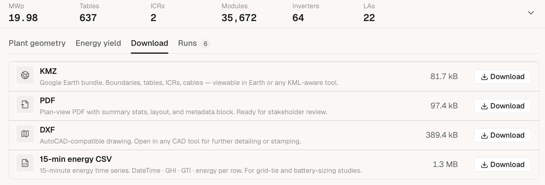
Open a completed run, then expand the bottom panel below the canvas and switch to the Download tab. If your layout used a custom hourly weather CSV, you'll see a fourth row labelled 15-min energy CSV below KMZ / PDF / DXF, each with its own Download button.

Download the file

Click Download on the 15-min energy CSV row and your browser saves <project>-<run>.csv.

Wait

The CSV is rendered by the cloud exporter alongside your KMZ / PDF / DXF, after the run finishes; the download is a single fetch, usually under 5 seconds.

Open or hand off

Open in Excel (works fine for a single year of 15-minute data — 35,040 rows), or in pandas / R / your modelling tool of choice.

Column reference

The CSV has four columns. Plant-level totals; no per-plot breakdown.

Row count: 4 × hours-in-your-weather-file. A standard 8,760-hour year produces 35,040 rows.

How Energy (kWh) is computed

For each 15-minute interval:

Energy_15min  =  capacity_kWp  ×  GTI / 1000  ×  PR  ×  LID  ×  0.25 h  ×  (1 + bifacial_gain)

• capacity_kWp — the sum of DC capacity across every plant in this project.
• PR — the Performance Ratio you see on Page 3 of the PDF report. PR captures inverter efficiency, DC / AC cable losses, soiling, temperature, mismatch, shading, availability, transformer loss, and other losses, per How yield is computed.
• LID — 1 − first_year_degradation_pct / 100, the year-1 light- induced degradation factor.
• 0.25 h — interval length.
• bifacial_gain — 0 for a monofacial module; for a bifacial module, the same flat rear-side gain applied to your headline year-1 number (see Bifacial modules).

Bifacial modules

For a bifacial module the headline year-1 energy applies a flat rear-side gain (the +X% you see on Page 3 of the PDF). Each 15-minute row carries that same gain, applied in proportion to its front-side output — so the rows still trace the real production curve, just lifted by the bifacial factor, and summing the Energy (kWh) column reconciles to your dashboard year-1 number. (Earlier exports were front-side only and summed ~X% below the dashboard; that's fixed.)

This is a flat-fraction distribution: SolarLayout models the rear-side gain as a constant share of front-side output, exactly as the headline does. True rear irradiance varies a little with sun angle through the day, so treat the per-interval split as an even approximation — the annual total and the production shape are right, but don't read a single interval's bifacial share as time-resolved physics.

Degradation handling

The CSV is a year-1, post-LID time series. Year-on-year annual degradation (typically 0.4 – 0.6 % / year over 25 years) is not baked into each row — the per-interval energy applies only the year-1 LID factor. The PDF's 25-year forecast applies annual degradation in its own pass; if you need degradation applied to the 15-minute series, multiply each row's energy by the year-N factor in your downstream model.

Common downstream uses

Grid-tie / curtailment

Filter Energy (kWh) against your evacuation cap (or sum the GTI column against a clear-sky reference) to estimate annual lost production when the grid back-feeds.

Battery / hybrid sizing

Resample to 1-minute or smooth across an hour to match your battery's response time, then run an SOC simulation against a load profile. The 15-minute grain is fine enough for arbitrage and peak-shaving sizing.

PPA / time-of-day tariff modelling

Group Energy (kWh) by hour of day → see when production peaks relative to your offtaker's load. Utility-scale typically peaks 11 AM – 2 PM in winter, 10 AM – 3 PM in summer — useful for ToD tariff negotiations.

Financial modelling

Aggregate Energy (kWh) to annual production, then apply your degradation curve and DC-coupled loss assumptions in the financial model.

File size and performance

• One year, 8,760 hourly inputs: 35,040 rows, typically ~1.5 – 2 MB.
• Two years of hourly inputs: 70,080 rows.

If you only need hourly aggregates, resample in one line:

import pandas as pd

df = pd.read_csv("my-layout.csv", parse_dates=["DateTime (UTC)"])
hourly = (
    df.set_index("DateTime (UTC)")
      .resample("1h")
      .sum()
)

What the CSV is NOT

• Not a per-plant breakdown. It's a plant-level total summed across every plant in the project. Per-plant numbers are in the PDF's per-plant table.
• Not multi-year. Row count = 4 × hours in your weather input. For lifetime production, use the PDF's 25-year forecast table.
• Not raw weather data. GHI is interpolated from your input weather CSV's hourly samples to 15-minute intervals; GTI is either read from your input (if present) or transposed from GHI.

When to use the CSV

The CSV is the right export when:

• You're doing time-series modelling downstream — grid-tie, curtailment, battery sizing, PPA / ToD analysis.
• You want to dig into specific time periods — monsoon underperformance, peak-summer derating, etc.
• You're handing off to a data science team for site-specific modelling.

For everything else — bid pack, client review, engineering hand-off — use PDF, KMZ, or DXF instead.